Writing a Lsd Model

Introduction

• Model equations: chunks of very simple programming language code for each Variable, much like the definition of a mathematical expression in a difference equation model;
• Model structure: a hierarchical collection of entities, called Objects. Each Object contains Variables, Parameters or other Objects; the Variables are associated to an equation, that can use the values of other Variables or Parameters of the model.
• Model configuration: the initial values used in a simulation run at the very first time step to kick off the simulation (e.g. the values of Parameters, the number of Objects, the number of time steps etc.). Configurations contain also information on the number of time steps, which data must be saved etc.

This tutorial lists the steps to be followed to create a Lsd model in general. Click on the step number for detailed instructions to create an example model.
 

Step	Operation	Instrument	Result
1	Design a model	Paper and  pencil	Decide one or few equations for a prototype of the model, and the entities to be represented. Sketch out the kind of results to investigate.
2	Create a new model	LMM	Generate an "empty" model, that is, all the technical requirement to build a model but with no equations' code contained in the equation file (see LMM help).
3	Insert equations	LMM	Fill the equation file with equations associated with Variables' labels.  Each equation is inserted independently, much like systems of difference equations. The programming knowledge required is limited to the logical/mathematical operations represented in the equation. See the help on Lsd equation coding.
4	Try to run the Lsd model program	LMM	Generate the Lsd model program, or, if errors occur, list the coding errors  (see LMM help). LMM attempts to create a model program by compiling the equation file. In case of syntactical errors in the equations' code LMM provides their list and location in the equation file.
5	Fix coding errors	LMM	Generate the Lsd model program (see LMM help). Using the list of errors provided after a failed compilation it is possible to quickly fix the errors in the equations code. Note that errors are listed along line numbers referring to the file where they occured. LMM shows you the line numbers in the editor, so it is easy to spot the location of the error.
6	Run the Lsd model	LMM	Access Lsd interfaces (see LMM help) LMM launches the Lsd model program. This contains, besides the equations' code used during a simulation run, all the interfaces to deal with a model.
7	Define model structure (Objects, Variables, Parameters)	Lsd	Generate a configuration (see Lsd help). To define a model structure the modeller needs only to type in the labels of the model elements. For a discussion on how to design a model structure see here.
8	Insert number of Objects and initial values	Lsd	Generate a configuration (see Lsd help). Given the definition of the model structure the Lsd interfaces generate suited windows to insert the numerical values required to start a simulation.
9	Define general simulation settings	Lsd	Generate a configuration (see Lsd help). Although provided by default, the modeller may want to determine the number of time steps per simulation run, the values to be saved, the series to be shown during the run, and other technical settings.
10	Run simulation	Lsd	Produce results, or logical errors. A simulation run produces the series for the data saved, but there may be "logical" errors, that is, legal C++ and Lsd code that cannot be executed given the state of the model in that moment. Examples of these errors are dead-locks (two equations requesting reciprocally to be computed before the other), or missing elements of the model (usually due to differences in spelling between the equation code and structure labels). Lsd captures these errors issuing suited messages (see Lsd help).
11	Fix logical errors	Lsd	Find offending code in the equations. In most cases the error messages issued by Lsd allow to quickly find the line in the equation's code that caused them, since the fatal errors issue messages in which the offending equation is reported (see Lsd help).
12	Analyse the Simulation Results	Lsd	Observe the data produced by a simulation (see Lsd help). The data saved during a simulation are loaded in the Analysis of Result module to produce plots, statistics, export data etc.
13	Test different configurations	Lsd	Produce different configurations. Generally starting from a fresh configuration (not one obtained after a simulation run), change the initial values of the simulation, saving the configuration with different values to test the behaviour of the model in different conditions (see here for changing model's values, or here for simulation settings).
14	Create the model report	Lsd	Create a HTML file reporting the model structure and the interdependencies between model elements. The report shows which item is used in each equation's code. The very equations' code is also included in the report. The report is extremely useful to understand the actual computations of a model.
15	Extend the model	LMM and Lsd	Add new elements to the model, adding also the equations for the new Variables. Each time a new equation is involved the model need to be re-compiled. See the Lsd equation manual for more detailed on the Lsd coding language.

The model you have created can be distributed to any Lsd user by just sending the directory where the model is contained. The user will have all the code and the documentation to repeat your simulation, understand them and possibly extending the model.
 

1 - Design a model

Let's consider a model where a group of firms compete on a market on the basis of the quality of their product. The driving equation is, for each firm:

• Sales_t = Sales_t-1*{1 + a*(Quality/AverageQuality_t-1 -1)}

• AverageQuality_t = sum_i{Quality_i * Sales_i/TotalSales}

• TotalSales_t  = sum_i{ Sales_i}

2 - Create a new model

3 - Insert equations

Let's use this structure to write the type in the equation the code for the Variable Sales (you can select the following text for the equations, up to the last "}" aftet the goto end;  statement, copying with the menu Edit/Copy in Netscape and then pasting in LMM). The equation code for Sales is:

EQUATION("Sales")
/*
Level of sales:
Sales[t]=Sales[t-1]*{1+a*(Quality/AverageQuality-1)}

The sales of a firm are adjusted in respect of the ratio between firm's own Quality and the
average quality.

*/

v[0]=V("a");
v[1]=VL("Sales",1);
v[2]=V("Quality");
v[3]=VL("AverageQuality",1);

RESULT( v[1]*(1+v[0]*(v[2]/v[3]-1)) )

Let's see what the equation does. The first line indicates that this code is the equation for the Variable Sales. Then we have placed a comment, without any use for the working of the equation, but helpful for documentation (this comment is automatically searched by the system and used in the model report).
The next 4 lines in the equation collect the data necessary to compute the value of Sales. The v[0], v[1], etc. are temporary C++ variables used to store intermediate results during computation. The Lsd function V("label") simply returns the value of the item "label") in the model. The VL("label", lag) function is the same as V("label"), but request the past value of "label", with 'lag' lags.
For example, in v[1] it is stored the value of the previous time step value of Sales.
The last line contains the result, that is, the numerical value that Sales will take after its equation has been computed.

Note that V("label") works identically whether the value searched is a Parameter (like a) or a Variable. Moreover, the function is identical for data that will be stored in different Objects. In fact, Sales is a Variable that we will place in an Object referring to firms, while AverageQuality will be located in another Object, Market.

Now we turn to write another equation. Place the cursor after the last line or before the first line of Sales (the order in which the equations' code is placed in the equation file does not matter).

The equation for TotalSales is:

EQUATION("TotalSales")
/*
Sum of the Sales from each Firm
*/

RESULT( SUM("Sales") )

The equation for AverageQuality is:
 

The equation initialise to 0 the value of v[0]. The equation is made of a cycle for, that is, a block of code (in between brakets) is repeated until a given logical condition is true (see LMM help on this topic). The header of the cycle (the line with for(...))  is made of three fields:

• a command to be executed before of the first run of the cycle, and never again;
• the condition for repeating the cycle;
• a command to be executed after each cycle and before the control of the condition.

The cycle for is composed by three fields, separated by a semi-colon:

• cur=p->search("Firm");

This means that the system must search for the first occurrence of the Object Firm, and store it in the temporary Object pointer cur;
• cur!=NULL;

This means that the cycle must be repeated as long as cur contains an Object, and be interrupted when cur is empty;
• cur=go_brother(cur)

This means that after a cycle, and before controlling for the condition in the second field, the pointer cur must be assigned the Object next to the Object it currently contains. The function go_brother(cur) returns an empty value (NULL) if there are no more Objects after cur.

EQUATION("AverageQuality")
/*
Average quality of products, weighted with the sales.

The equation scans all the Object Firm summing up the product Sales x Quality and dividing for
the total sales.
*/
v[0]=V("TotalSales");
v[1]=0;
CYCLE(cur, "Firm")
 {//assign to pointer 'cur' all the Firm

  v[2]=VS(cur,"Sales"); //compute Sales for the current Firm
  v[3]=VS(cur,"Quality"); //compute Quality for the current Firm
  v[1]=v[1]+v[2]*v[3]; //cumulate the product Sales times Quality
 }

RESULT(v[1]/v[0] )

This equation deserves some attention. Firstly, we store in v[0] the value of total sales. Then, we initialize v[1] to 0. The next lines contain a cycle so that make a temporary "pointer" (that is, a temporary variable containing Objects instead of numerical values) to contain cyclically all the Objects named Firm. The cycle repeat the commands between the '{' and '}' for all the Object Firm in the mdoel. In each cycle we make three operations: collect the value of Sales and Quality for the firm contained in the pointer,  add their product to v[1].
Note that we use the Lsd function VS(pointer, "label"). This function asks specifically the value of "label" to the Object 'pointer', instead of generally search one copy of "label" in the model.

Now you have inserted the equations for your model. For more information on the Lsd equations' language see the Lsd help on this).

return to the tutorial list

4 - Create the Model program

5 - Fix the compilation errors

6 - Access the Lsd interfaces

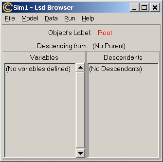
When the Lsd model starts it is empty. That is, there is no configuration loaded in the model program, although the program contains the equations' code embedded in its C++ core. The interface is composed by the Browser, which shows one Object (the Object shown is indicated in red along "Object's label"). The Lsd Browser shows two list boxes, for the set of Variables, on the left, and for the Objects descending from the currently shown one, on the left. Currently, the Browser shows the Object Root, included by default in any Lsd model, which contains no Variables and no descending Objects.
The Lsd model program starts also a new window, called Log. This will contain messages from the system, when necessary. For the moment you can ignore it.
The Browser contains several menus. Modellers are interested only in the menu Model to determine the model structure, while the other menus are used to manage different aspects of the simulation that also users may be interested in changing (like initial values, number of time steps, etc.). The structure of the model and the initializations are saved in configurations files (extension .lsd) that can be loaded to run directly a simulation run.

return to the tutorial list

7 - Define the model structure

• Choose the item Add Descending Obj. in menu Model to add an Object to Root. Type the label Market and press Ok (you may add a description, but for the moment leaves the box empty). Now the Browser shows Market in the list of descendants. Notice that a new window has appeared, titled Lsd Model Structure. This is a graphical representation of the model (ignoring Root).
• Double-click on Market to move the Browser to show Object Market. If you typed the wrong label instead of Market you can click on its name in the header of the Browser window. If you remove completely the label, leaving an empty string, the Object is removed altogether.
• Market is created with no Variable or Parameters. We need Market to contain one Parameter, a, and two Variables, TotalSales and AverageQuality. Choose the item Add a Parameter in menu Model and type a. Insert the Variable TotalSales choose menu item Model/Add a Variable. When adding the Variable AverageQuality set to 1 the lag desired. This is because we need to use AverageQuality with lag 1 (in the equation for Sales), and this must be signalled when the Variable is created. Notice that the Browser window will list in the Variables list box the elements added.
• Control that the Browser appears as below (the order of Variables and Parameters does not matter):

• The list of Variables shows the label of the items followed by (P), if it is a Parameter, and by an integer if it is a Variable. The integer indicate the number of lag values that the Variable must kept during a simulation step.
• If you made a mistake inserting an element, double-click on the wrong item. You are shown the list of options for the item. Double-click on the label of the item to edit it to fix the error. Inserting an empty label will remove the item altogether.
• The order in which the items appear in the Variables' list of an Object is not relevant (it follows the order of insertion).
• Create now the Object Firm, as descending from Market (choose item Add Descending Obj. in menu Model and type Firm). The Browser will list Firm as descending from Market. Double-click on Firm moving the Browser to show this Object. Notice that the Lsd Model Structure window has been updated showing Market as containing Firm.
• In Firm (when the Browser shows it), use the same process (menu Model and Add a Variable or Add a Parameter) to create the Variable Sales (it needs one lag) and the Parameter Quality.

8 - Insert initial values and the number of Objects

Now we have the model configured with 1 instance of Object Market and 10 Object Firm. To run a simulaiton we need to determine the values of the Paremeters and of the lagged Variables to be used at the first time step of a simulation run, that is the initial values. Setting the number of Objects can be done for the whole model at once. Instead, setting the initial values must be done for one Object type per time. Move the Browser to show the Object Firm (you can double-click on the symbol representing Firm in the graphical representation of the model). Choose the item Initial Values in menu Data. The window is like a spreadsheet, listing the different instances of Objects on the columns and the Parameters or lagged Variables on the lines. You can manually type in each cell a number (pressing Return on your keyboard to move to the next cell), or use the Set All button to set the whole values for a line (see the Lsd manual on this). For the Objects Firm we need to set the lagged values of Sales and the level of Quality. Set the same value for Sales for all firms (say 100). To do this using the Set All button, type 100 and select the option Equal To. For Quality set increasing values from 1, 1.1, 1.2 etc. To do this, select the option Increasing, and type 1 as starting value and 0.1 as step.

Click on Ok when you have finished to set the initial values for Objects Firm, move the Browser to show the Object Market (click on the label Market in the Browser on the left of the text "Descending from: ..."), and choose Initial Values in menu Data. You can obtain the same result by clicking with the right button of the mouse on the symbol for Market in the graphical representation. Notice that the Variable TotalSales does not appear in the window. In fact, this Variable does not need to be initialized, since it is never used as lagged value. Type 0.05 for the Parameter a and 1.5 for AverageQuality with lag 1.
return to the tutorial list

9 - General Simulation Settings

10 - Run the simulation

If there are errors the simulation is interrupted immediately, or the Lsd error manager issue few messages offering the modeller with several possibilities to investigate the error (see Fix logical errors below). If the simulation runs smoothly, you will see a new window, the Run Time Plot, showing the series of the data set with this option (Sales in the example). If you did not set any Variable to appear in the Run Time Plot, then the Log window will signal all steps that have been successfully completed.
During a simulation run the Log window can be used to control the simulation, using the four buttons in the lower part of the window:

• Stop: end the simulation when the current time step is finished;
• Fast: continue the simulation without issuing the time step lines in the Log window (only if there is no Run Time Plot windows);
• Observe: return to show the time step completed (only if there is no Run Time Plot windows);
• Debug: set on the Debug Mode, temporarily interrupting the simulation and allowing to explore the status of the model.

Although it is not strictly necessary for writing Lsd models, it may be interesting to know what happens when a simulation is run. The operations of a simulation run are:

1. Save the configuration file (beware that every change to the model overwrites the pre-existing configuration)
2. Set the simulation time counter to 1
3. Select the Root Object as current Object
4. Compute the equation for all the Variables in the current Object
5. Set the descendants of the current Object as new current Object and return to 4.
6. (when all Objects of the model have been explored) increase the time counter and return to 3.

When a lower Variable already computed is reached by the standard simulation cycle, or it is requested again by another Variable, Lsd does not re-compute it, but uses the value already computed the first time in that time step.
Modellers can also decide to use Variables that, instead having an equation assigned, has a function. This is identical to an equation, but includes also few lines such that the value of the Variable is recomputed as many times as it is requested, even many times during a time step.

return to the tutorial list

11 - Fix logical errors

Data not loaded

Data for XXX in Object YYY not loaded

This happen either when a Parameter or lagged Variable is inserted, or when the number of Objects is increased, but the user did not set any initial value for it. In both cases Lsd assign a default value that must be, at least, confirmed before being able to run a simulation.
To fix the error re-load the configuration (menu File/Re-Load). Move the Browser to show the Object YYY containing the un-initialized elements. Choose item Initial Values in menu Data. Even if the data are not changed, only opening this window is considered as a confirmation of the values presented.

Variable not found

Equation for XXX not found

it means that the Variable defined in the model configuration does not correspond to any equation block in the equation file. This error is also caused if you defined a Variable instead of a Parameter (to Lsd, it is a Variable without equation). For example, if you defined a as a Variable it appears as
a (0)
in the left list box in Market, instead of
a (P)
as it should be for Parameters. See below how to correct this error.

If the error is:

Search for XXX failed in YYY
Fatal error detected at time 1.
Offending code contained in the equation for Variable: ZZZ

it means that the Variable (or Parameter) XXX requested in the equation for ZZZ was not found. You likely mispelled XXX in the equation's code.

To correct the error you need either to change the equations code, or to change the label of the element in the model structure. In any case, close the Lsd model program (choosing Abort if the error message is of the second type). You can change the equations' code, if necessary, using LMM. Save the equations' file (menu File/Save) and run the Lsd model program (menu Model/Run). When the Lsd model program starts, load the configuration (menu File/Load) and choose the configuration file that caused the error. Now the model is defined exactly as when you started the simulation, but with the fixed equation code. If you want to edit the model structure definition (e.g. change the label) move the Browser to show the Object containing the Variable to be changed. Double-click on it, and, in the option window, double-click on its label to change as necessary. After the changes try to run the simulation again (menu Run/Run).
 

Lag error

Lag error: Variable XXX requested lag K but available only H

This means that the Variable XXX in the equation was requested with a lag superior than that available (typically, it is requested with 1 lag, but it was defined without any lag, or lag 0). Again, it may be an error in the equations' code, or in the model structure definition. Follow the instructions on how to correct this error.
 

Dead lock error

Fatal error detected at time 1.
Offending code contained in the equation for Variable: Sales

List of Variables currently under computation.
(the first-level Variable is computed by the simulation manager,
while possible other Variables are triggered by the lower level ones
because necessary for completing their computation)

Level Variable Label
3 Sales
2 TotalSales
1 AverageQuality
0 Lsd Simulation Manager

The lines highlighted show the two Variables involved in the dead-lock.
To fix the error set one call with a lag, according to the logic you want to use in the model.

return to the tutorial list

12 - Analyse the Simulation Results

13 - Test different configurations

14 - Create Model Report

To create the report it is necessary to tell the system the equation file name, menu Model item Equation File, and indicating the filename suggested in the resulting window. Lsd model programs permit to add to each item a textual description, that appear in their option window and are used in the model report. However, it is also possible to request the system to automatically induce some of the relevant information. To do this, use the command in menu Model / Generate Automatic Documentation. After this, click on a Parameter or a Variable to see the results.

Then choose the item Create Model Report in menu Model and the system pops up a window where the modeller can choose the options concerning the report. Confirming the creation of the report makes the system create the report's file (or overwrite the existing file). After the creation the report is shown. It is always possible to access the report from its indication in the menu Help (obviously, only if available).
return to the tutorial list

15 - Extend the model

Close the Lsd model program and return to LMM, open the equation file for the model (menu Model/Show Equation), and place the cursor in a legal position for a Lsd equation (within the lines MODELBEGIN and MODELEND and outside the block for an existing equation).

Press the keys Ctrl+Shift+e to insert an equation (or use the normal way through the menu Model/Insert Lsd Scripts), for the Variable "ms".

The block for the equation is:

EQUATION("ms")
/*
Market shares
*/
v[0]=V("Sales");
v[1]=V("TotalSales");

RESULT( v[0]/v[1])
 

Now you have inserted the new equation saying that the market shares (Variable "ms") must be computed as the ratio between Sales and TotalSales. The whole equation should be like:

Save the equation file (menu File/Save, or press Ctrl+s), and run the model, menu Run/Run. The system automatically acknowledges that the file is changed, and therefore recompiles the whole Lsd model program.

When the Lsd Browser window appears, open one of the configuration files (menu File/Load). Note that you may run the model as before since the new code does not interfere with the previous equations.

Move the Browser to point to the Object Firm (double-click on the symbol for Firm in the graphical representation). There insert the new Variable "ms": choose menu Model/Add a Variable (or press Ctrl+v), and type "ms", with 0 lags.

As last operation, double-click on the newly insereted "ms" Variable in the list of Variables for Firm and check on the To Save option, so to include the values of the market shares Variables in the data saved during the simulation runs.

Now you can run a simulation and observe the results
return to the tutorial list